Demand estimation and forecastingThe first question which arises is, what is the difference between demand estimation and demand forecasting? The answer is that estimation attempts to quantify the links between the level of demand and the variables which determine it. Forecasting, on the other hand, attempts to predict the overall level of future demand rather than looking at specific linkages. For this reason the set of techniques used may differ, although there will be some overlap between the two.In general, an estimation technique can be used to forecast demand but a forecasting technique cannot be used to estimate demand. A manager who wishes to know how high demand is likely to be in two years’ time might use a forecasting technique. A manager who wishes to know how the firm’s pricing policy could be used to generate a given increase in demand would use an estimation technique.The firm needs to have information about likely future demand in order to pursue optimal pricing strategy. It can only charge a price that the market will bear if it is to sell the product. On one hand, over-optimistic estimates of demand may lead to an excessively high price and lost sales. On the other hand, over-pessimistic estimates of demand may lead to a price which is set too low resulting in lost profits. The more accurate, information the firm has, the less likely it is to take a decision which will have a negative impact on its operations and profitability.The level of demand for a product will influence decisions, which the firm will take regarding the non-price factors that form part of its overall competitive strategy.For example, the level of advertising it carries out will be determined by the perceived need to stimulate demand for the product. As advertising expenditure represents an additional cost to the firm, unnecessary spending in this area needs to be avoided. If the firm’s expectations about demand are too low it may try to compensate by spending large sums on advertising, money which in this instance may be, at least, partly wasted. Alternatively it may decide to redesign the product in response to this, thus incurring unnecessary additional costs in the form of research and development expenditure.In the previous unit, demand analysis was introduced as a tool for managerial decision-making. For example, it was shown that knowledge of price and cross elasticities can assist managers in pricing and that income elasticities provide useful insights into how demand for a product will respond to different macroeconomic conditions. We assumed that these elasticities were known or that the data were already available to allow them to be easily computed. Unfortunately, this is not usually the case. For many business applications, the manager who desires information about elasticities must develop a data set and use statistical methods to estimate a demand equation from which the elasticities can then be calculated. This estimated equation could then, also be used to predict demand for the product, based on assumptions about prices, income, and other factors. In this unit the basic techniques of demand estimation and forecasting are introduced. ESTIMATING DEMAND USING REGRESSION ANALYSIS The basic regression tools discussed in Block 1 can also be used to estimatedemand relationships. Consider a small restaurant chain specializing in Chinesedinners. The business has collected information on prices and the average numberof meals served per day for a random sample of eight restaurants in the chain.These data are shown below. Use regression analysis to estimate the coefficients of the demand function Qd = a + bP. Based on the estimated equation, calculate thepoint price elasticity of demand at mean values of’ the variables. |
|
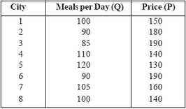
Solution : The mean values of the variables are Q = 100 and P = 160. The other data needed to calculate the coefficients of the demand equation are shown below.
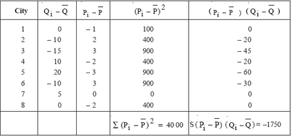
As shown, the sum of the ( 2Pi − P) is 4000 and the sum of the ( Pi − P)( Q Qi − ) is –1750 Thus, using the equations for calculating
bˆ and aˆ ,bˆ= –175/40 = –.4375 and aˆ = 100 – (.4375)(160) = 170 .Hence, the estimated demand equation is Qd = 170 – 4.375*P. Recall from the previous unit that the formula for point price elasticity of demand is Ep = (dQ/dP)(P/Q). Based on the estimated demand function, dQ/dP = –.4375. Thus, using the mean values for the price and quantity variables, Ep = (–.4375)(160/100) =– 0.7.
bˆ and aˆ ,bˆ= –175/40 = –.4375 and aˆ = 100 – (.4375)(160) = 170 .Hence, the estimated demand equation is Qd = 170 – 4.375*P. Recall from the previous unit that the formula for point price elasticity of demand is Ep = (dQ/dP)(P/Q). Based on the estimated demand function, dQ/dP = –.4375. Thus, using the mean values for the price and quantity variables, Ep = (–.4375)(160/100) =– 0.7.
EVALUATING THE ACCURACY OF THE REGRESSION EQUATION - REGRESSION STATISTICS
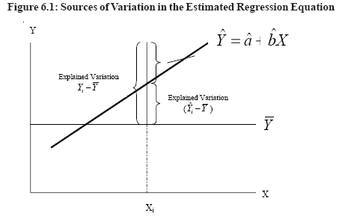
Once the parameters have been estimated, the strength of the relationship between the dependent variable and the independent variables can be measured in two ways. The first uses a measure called the coefficient of determination, denoted as R2, to measure how well the overall equation explains changes in the dependent variable. The second measure uses the t-statistic to test the strength of the relationship between an independent variable and the dependent variable.Testing Overall Explanatory Power : Define the squared deviation of any Yi from the mean of Y [i.e., (Yi–Y)2] as the variation in Y. The total variation is found by summing these deviations for all values of the dependent variable as total variation = S (Yi–Y)2 Total variation can be separated into two components: explained variation and unexplained variation. These concepts are explained below, for each Xi value,compute the predicted value of Yi (denoted as i Yˆ ) by substituting Xi in the estimated regression equation:i Yˆ= i X bˆ aˆ +The squared difference between the predicted value Yi and the mean value Y[i.e.,( i Yˆ –Y)2] defined as explained variation. The word explained means that the deviation of Y from its average value is Y the result of (i.e., is explained by) changes in X. For example, in the data on total output and cost used previously, one important reason the cost values are higher or lower than Yis because output rates(Xi) are higher or lower than the average output rate.Total explained variation is found by summing these squared deviations, that is,total explained variation = Σ − i Yˆ (Unexplained variation is the difference between Yi and . That is, part of the deviation of Yi from the average value (Y) is "explained" by the independent variable, X. The remaining deviation, Yi - i Yˆ , is said to be unexplained. Summing the squares of these differences yields total unexplained variation = Σ(Yi − Yˆ1)2.The three sources of variation are shown in Figure 6.1.
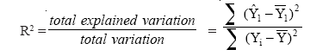
The coefficient of determination (R2) measures .the proportion of total’ variation in the dependent variable that is "explained" by the regression equation. That is,
The value of R2 ranges from zero to 1. If the regression equation explains none of the variation in Y (i.e., there is no relationship between the independent variables and the dependent variable), R2 will be zero. If the equation explains all the variation (i.e., total explained variation = total variation), the coefficient of determination will be 1. In general, the higher the value of R2, the "better" the regression equation. The term fit is often used to describe the explanatory power of the estimated equation. When R2 is high, the equation is said to fit the data well. A low R2 would be indicative of a rather poor fit.
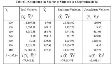
How high must the coefficient of determination be in order that a regression equation be said to fit well? There is no precise answer to this question. For some relationships, such as that between consumption and income over time, one might expect R2 to be at least 0.95. In other cases, such as estimating the relationship Demand Estimation and Forecasting between output and average cost for fifty different producers during one production period, an R2 of 0.40 or 0.50 might be regarded as quite good.Based on the estimated regression equation for total cost and output, that is,i Yˆ = 87.08 + 12.21X1 the coefficient of determination can be computed using the data on sources of variation shown in Table 6.1.
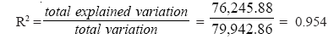
The value of R2 is 0.954, which means that more than 95 percent of the variation in total cost is explained by changes in output levels. Thus the equation would appear to fit the data quite well.
Evaluating the Explanatory Power of Individual Independent Variables
The t-test is used to determine whether there is a significant relationship between the dependent variable and each independent variable. This test requires that the standard deviation(or standard error) of the estimated regression coefficient be computed. The relationship between a dependent variable and an independent variable is not fixed because the estimate of b will vary for different data samples.
The standard error of bˆ from one of these regression equations provides anestimate of the amount of variability in b. The equation for this standard error is
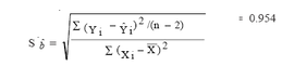
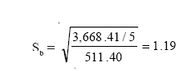
where n is the number of observations. For the production-cost example used in this section, n = 7 and the standard error of bˆ is
The least-squares estimate of bˆ is said to be an estimate of the parameter b. But it is known that bˆ is subject to error and thus will differ from the true value of the parameter b. That is why bˆ is called an estimate. Because of the variability in bˆ , it sometimes is useful to determine a range or interval for the estimate of the true parameter b. Using principles of statistics, a 95 percent confidence interval estimate for b is given by the equation bˆ + tn-k-1S bˆ
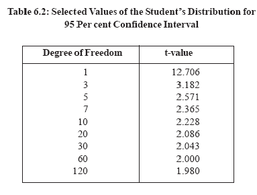
where tn-k-1 represents the value of a particular probability distribution known asstudent’s distribution. The subscript (n -k -1) refers to the number of degrees offreedom, where n is the number of observations or data points and k is the numberof independent variables in the equation. An abbreviated list of t-values for use inestimating 95 percent confidence intervals is shown in Table 6.4. In the examplediscussed here, n = 7 and k = 1, so there are five (i.e., 7 -1 -1) degrees of freedom,and the value of t in the table is 2.571. Thus, in repeated estimations of the outputcostrelationship, it is expected that about 95 percent of the time such that the truevalue of parameter b will lie in the interval defined by the estimated value of b plus or minus 2.571 times the standard error of b. For the output-cost data, the 95 percent confidence interval estimate would be 12.21+ 2.571(1.19) or from 9.15 to 15.27. This means that the probability that the true marginal relationship between cost and output (i.e., the value of b) within this range is 0.95. If there is no relationship between the dependent and an independent variable, the parameter b would be zero. A standard statistical test for the strength of the
relationship between Y and X is to check whether the 95 percent confidence interval includes the value zero. If it does not, the relationship between X and Y as measured by bˆ is said to be statistically significant. If that interval does include zero, then 6 is said to be non significant, meaning that there does not appear to be a strong relationship between the two variables. The confidence interval for in bˆ the output-cost example did not include zero, and thus it is said that bˆ , an estimate of marginal cost, is statistically significant or that there is a strong relationship between cost and rate of output. Another way to make the same test is to divide the estimated coefficient (bˆ ) by its standard error. The probability distribution of this ratio is the same as Student’s t distribution; thus this ratio is called a t-value. If the absolute value of this ratio is equal to or greater than the tabled value of t for n - k - 1 degrees of freedom, bˆ is said to statistically significant. Using the output-cost data, the t-value is computed to be
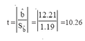
Because the ratio is greater than 2.571, the value of the t-statistic from Table 6.2, it is concluded that there is a statistically significant relationship between cost and output. In general, if the absolute value of the ratio bˆ / bˆ S is greater than the value from the table for n -k -1 degrees of freedom, the coefficient bˆ is said to be statistically significant.
The standard error of the equation is used to determine the likely accuracy with which we can predict the value of the dependent variable associated with particular values of the independent variables. As a general principle, the smaller the value of the standard error of the equation, the more accurate the equation is and hence the more accurate any predictions made from it will be. To put this in another way, the standard error represents the standard deviation of the dependent variable about the regression line. Thus the smaller the value, the better the fit of the equation to the data and the closer the estimate will be to the true regression line. Conversely, the larger the standard error, the bigger the deviation from the regression line and the less confidence that can be put in any prediction arising from it. The standard error of the coefficient works along similar lines. It gives an indication of the amount of confidence that can be placed in the estimated regression coefficient for each independent variable. Again, the smaller the value, the greater the confidence that can be placed in the estimated coefficient and vice versa. Finally, the t-test provides a further measurement of the accuracy of the regression coefficient for each of the independent variables.A value of t greater than or equal to 2 generally indicates that the calculated
coefficient is a reliable estimate, while a value of less than 2 indicates that the coefficient is unreliable. (Note: This also partly depends, however, on the number of data observations on which the equation is based so that t-test tables need to be used in order to ensure an accurate interpretation of this statistic.)
coefficient is a reliable estimate, while a value of less than 2 indicates that the coefficient is unreliable. (Note: This also partly depends, however, on the number of data observations on which the equation is based so that t-test tables need to be used in order to ensure an accurate interpretation of this statistic.)
THE MARKETING APPROACH TO DEMAND MEASUREMENT
The vast majority of business decisions involve some degree of uncertainty and managers seldom know exactly what the outcomes of their choices will be. One approach to reducing the uncertainty associated with decision making is to devote resources to forecasting. Forecasting involves predicting future economic conditions and assessing their effect on the operations of the firm. Frequently, the objective of forecasting is to predict demand. In some cases,managers are interested in the total demand for a product. For example, the decision by an office products firm to enter the home computer market may be determined by estimates of industry sales growth. In other circumstances, the projection may focus on the firm’s probable market share. If a forecast suggests that sales growth by existing firms will make successful entry unlikely, the company may decide to look for other areas in which to expand.Forecasts can also provide information on the proper product mix. For an automobile manufacturer such as Maruti Udyog, managers must determine the number of Esteems versus Zens to be produced. In the short run, this decision is largely constrained by the firm’s existing production facilities for producing each kind of car. However, over a longer period, managers can build or modify production facilities. But such choices must be made long before the vehicles begin coming off the assembly line. Accurate forecasts can reduce the uncertainty caused by this long lead time. For example, if the price of petrol is expected to increase, the relative demand for Zens or compact cars is also likely to increase.Forecasting is an important management activity. Major decisions in large businesses are almost always based on forecasts of some type. In some cases, the forecast may be little more than an intuitive assessment of the future by those involved in the decision. In other circumstances, the forecast may have required thousands of work hours and lakhs of rupees. It may have been generated by the firm’s own economists, provided by consultants specializing in forecasting, or be
based on information provided by government agencies. Forecasting requires the development of a good set of data on which to base the analysis. A forecast cannot be better than the data from which it is derived. Three important sources of data used in forecasting are expert opinion, surveys, and market experiments.
Expert Opinion
The collective judgment of knowledgeable persons can be an important source of information. In fact, some forecasts are made almost entirely on the basis of the personal insights of key decision makers. This process may involve managers conferring to develop projections based on their assessment of the economic conditions facing the firm. In other circumstances, the company’s sales personnel may be asked to evaluate future prospects. In still other cases, consultants may be employed to develop forecasts based on their knowledge of the industry. Although predictions by experts are not always the product of "hard data," their usefulness should not be underestimated. Indeed, the insights of those closely connected with an industry can be of great value in forecasting.Methods exist for enhancing the value of information elicited from experts. One of the most useful is the Delphi technique. Its use can be illustrated by a simple example. Suppose that a panel of six outside experts is asked to forecast a firm’s sales for the next year. Working independently, two panel members forecast an 8 percent increase, three members predict a 5 percent increase, and one person predicts no increase in sales. Based on the responses of the other individuals, each expert is then asked to make a revised sales forecast. Some of those expecting rapid sales growth may, based on the judgments of their peers, present less optimistic forecasts in the second iteration. Conversely, some of those predicting
slow growth may adjust their responses upward. However, there may also be some panel members who decide that no adjustment of their initial forecast is warranted.Assume that a second set of predictions by the panel includes one estimate of a 2 percent sales increase, one of 5 percent, two of 6 percent, and two of 7 percent. The experts again are shown each other’s responses and asked to consider their forecasts further. This process continues until a consensus is reached or until further iterations generate little or no change in sales estimates. The value of the Delphi technique is that it aids individual panel members in assessing their forecasts. Implicitly, they are forced to consider why their judgment differs from that of other experts. Ideally, this evaluation process should generate more precise forecasts with each iteration.One problem with the Delphi method can be its expense. The usefulness of expert opinion depends on the skill and insight of the experts employed to make predictions. Frequently, the most knowledgeable people in an industry are in a position to command large fees for their work as consultants or they may beemployed by the firm, but have other important responsibilities, which means thatthere can be a significant opportunity cost in involving them in the planning process.Another potential problem is that those who consider themselves experts may beunwilling to be influenced by the predictions of others on the panel. As a result,there may be few changes in subsequent rounds of forecasts.
SurveysSurveys of managerial plans can be an important source of data for forecasting.The rationale for conducting such surveys is that plans generally form the basis forfuture actions. For example, capital expenditure budgets for large corporations areusually planned well in advance. Thus, a survey of investment plans by suchcorporations should provide a reasonably accurate forecast of future demand forcapital goods.Several private and government organizations conduct periodic surveys. The annualNational Council of Applied Economic Research (NCAER) survey of MarketInformation of Households is well recognized. Many private organizations likeORG-MARG and TNS-MODE conduct surveys relating to consumer demandacross certain geographical areas.If data from existing sources do not meet its specific needs, a firm may conduct itsown survey. Perhaps the most common example involves companies that areconsidering a new product or making a substantial change in an existing product.But with new or modified products, there are no data on which to base a forecast.One possibility is to survey households regarding their anticipated demand for theproduct. Typically, such surveys attempt to ascertain the demographiccharacteristics (e.g., age, education, and income) of those who are most likely tobuy the product and find how their decisions would be affected by different pricingpolicies.Although surveys of consumer demand can provide useful data for forecasting,their value is highly dependent on the skills of their originators. Meaningful surveysrequire careful attention to each phase of the process. Questions must be preciselyworded to avoid ambiguity. The survey sample must be properly selected so thatresponses will be representative of all customers. Finally, the methods of surveyadministration should produce a high response rate and avoid biasing the answersof those surveyed. Poorly phrased questions or a nonrandom sample may result indata that are of little value.Even the most carefully designed surveys do not always predict consumer demandwith great accuracy. In some cases, respondents do not have enough information todetermine if they would purchase a product. In other situations, those surveyedmay be pressed for time and be unwilling to devote much thought to their answers.Sometimes the response may reflect a desire (either conscious or unconscious) toput oneself in a favorable light or to gain approval from those conducting thesurvey. Because of these limitations, forecasts seldom rely entirely on results ofconsumer surveys. Rather, these data are considered supplemental sources ofinformation for decision making.
Market Experiments
A potential problem with survey data is that survey responses may not translateinto actual consumer behavior. That is, consumers do not necessarily do what theysay they are going to do. This weakness can be partially overcome by the use ofmarket experiments designed to generate data prior to the full-scale introduction ofa product or implementation of a policy.To set up a market experiment, the firm first selects a test market. This market may consist of several cities; a region of the country, or a sample of consumers taken from a mailing list. Once the market has been selected, the experiment mayincorporate a number of features. It may involve evaluating consumer perceptions of a new product in the test market. In other cases, different prices for an existing product might be set in various cities in order to determine demand elasticity. A third possibility would be a test of consumer reaction to a new advertising campaign.There are several factors that managers should consider in selecting a test market.First, the location should be of manageable size. If the area is too large, it may beexpensive and difficult to conduct the experiment and to analyze the data. Second,the residents of the test market should resemble the overall population of India inage, education, and income. If not, the results may not be applicable to other areas.Finally, it should be possible to purchase advertising that is directed only to thosewho are being tested.Market experiments have an advantage over surveys in that they reflect actualconsumer behavior, but they still have limitations. One problem is the risk involved.In test markets where prices are increased, consumers may switch to products ofcompetitors. Once the experiment has ended and the price reduced to its originallevel, it may be difficult to regain those customers. Another problem is that the firmcannot control all the factors that affect demand. The results of some marketexperiments can be influenced by bad weather, changing economic conditions, orthe tactics of competitors. Finally, because most experiments are of relatively shortduration, consumers may not be completely aware of pricing or advertisingchanges. Thus their responses may understate the probable impact of those changes.
Activity 2
What are the major marketing approaches to demand measurement?
DEMAND FORECASTING TECHNIQUES
Time-series analysis
Regression analysis, as described above, can be used to quantify relationshipsbetween variables. However, data collection can be a problem if the regression model includes a large number of independent variables. When changes in avariable show discernable patterns over time, time-series analysis is an alternative method for forecasting future values.The focus of time-series analysis is to identify the components of change in thedata. Traditionally, these components are divided into four categories:1. Trend2. Seasonality3. Cyclical patterns4. Random fluctuationsA trend is a long-term increase or decrease in the variable. For example, the timeseries of population in India exhibits an upward trend, while the trend forendangered species, such as the tiger, is downward. The seasonal componentrepresents changes that occur at regular intervals. A large increase in sales ofumbrellas during the monsoon would be an example of seasonality.Analysis of a time series may suggest that there are cyclical patterns, defined assustained periods of high values followed by low values. Business cycles fit thiscategory. Finally, the remaining variation in a variable that does not follow anydiscernable pattern is due to random fluctuations. Various methods can be usedto determine trends, seasonality, and any cyclical patterns in time-series data.However, by definition, changes in the variable due to random factors are notpredictable. The larger the random component of a time series, the less accuratethe forecasts based on those data.
Trend Projection
One of the most commonly used forecasting techniques is trend projection. As thename suggests, this approach is based on the assumption that there is an identifiable trend in a time series of data. Trend projection can also be used as the starting pointfor identifying seasonal and cyclical variations.Table 6.3 is a time series of a firm’s quarterly sales over a three-year time span.These data are used to illustrate graphical and statistical trend projection and also to describe a method for making seasonal adjustments to a forecast.
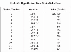
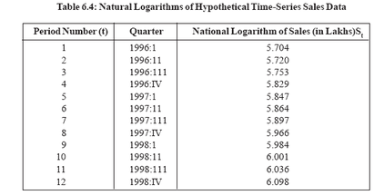
Statistical Curve Fitting Basically, this involves using the ordinary least-squares concept developed above to estimate the parameters of the equation. Suppose that an analyst determines that a forecast will be made assuming that there will be a constant rate of change in sales from one period to the next. That is, the firm’s sales will change by the same amount between two periods. The time-series data of Table 6.4 are to be used to estimate that rate of change.Statistically, this involves estimating the parameters of the equation St = So + bt where S denotes sales and t indicates the time period. The two parameters to be estimated are So and b. The value of So corresponds vertical intercept of the line and the parameter b is the constant rate of change and corresponds to the slope.Many hand calculators can estimate the parameters of equation. Specific procedures vary from model to model, but usually the only requirement is that the user input the data and push one or two designated keys. The machine then returns the estimated parameters. For the data of Table 6.3, the quarters would have to be inputted as sequential numbers starting with 1. That is, 1996: I would be entered as 1, 1996: II would be entered as 2, and so forth. Based on the data from the table, the equation is estimated as Sf = 281.394 + 12.811t. The interpretation of the equation is that the estimated constant rate of increase in sales per quarter is Rs. 12.811 lakhs. A forecast of sales for any future quarter, St, can be obtained by substituting in the appropriate value for t. For example, the third quarter of 1999 is the 15th observation of the time series. Thus, the estimated sales
for that quarter would be 281.394 + 12.811(15), or Rs. 473.56 lakhs. Now suppose that the individual responsible for the forecast wants to estimate a
percentage rate of change in sales. That is, it is assumed that sales will increase by a constant percent each period. This relationship can be expressed mathematically as St= St-1(1 + g)
Similarly,St-l = St-2(1 + g) where g is the constant percentage rate of change, or the growth rate. These two equations imply that St = St-2(1 + g)2
and, in general,St = So(l + g)t As shown, the parameters of this equation cannot be estimated using ordinary least squares. The problem is that the equation is not linear. However, there is a simple transformation of the equation that allows it to be estimated using ordinary least squares.Take logs, the result is ln St = ln [So(l + g)t] But the logarithm of a product is just the sum of the logarithms. Thus ln St = ln So + ln[(l + g)t]
The right-hand side of the equation can be further simplified by noting that ln [(l + g)t] = t[ln(l + g)] Hence ln St = ln So + t(ln(l + g)]
This equation is linear in form. This can be seen by making the following substitutions:Yt = ln St Yo= ln Sob = ln(l + g).Thus the new equation isYt = Yo + bt which is linear.The parameters of this equation can easily be estimated using a hand calculator. The key is to recognize that the sales data have been translated into logarithms.Thus, instead of SI, it is in Si that must be entered as data. However, note that the t values have not been transformed, Hence for the first quarter of 1996, the data to be entered are In 300 = 5.704 and l; for the second quarter, In 305 = 5.720 and 2;and so forth. The transformed data are provided in Table 6.4
Using the ordinary least-squares method, the estimated parameters of the equation based on the data from Table 6.5 are Yt = 5.6623 + 0.03531
But these parameters are generated from the logarithms of the data. Thus, for interpretation in terms of the original data, they must be converted back based on the relationships In So = Yo= 5.6623 and 1n (1 + g) = b = 0.0353. Taking the antilogs yields So = 287.810 and 1 + g = 1.0359. Substituting these values for So and 1 + g back into the original equation gives St = 287.810(1.0359)t where 287.810 is sales (in lakhs of rupees) in period 0 and the estimated growth rate, g, is 0.0359 or 3.59 per cent. To forecast sales in a future quarter, the appropriate value of 1 is substituted into the equation. For example, predicted sales in the third quarter of 1999 (i.e., the fifteenth quarter) would be 287.810 (1.0359)15, or Rs 488.51 lakhs.
Seasonal Variation in Time-Series Data
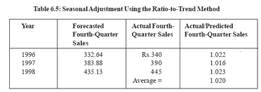
Seasonal fluctuations in time-series data are not uncommon. In particular, a largeincrease in sales for the fourth quarter is a characteristic of certain industries.Indeed, some retailing firms make large amounts of their total sales during theDiwali period. Other business activities have their own seasonal sales patterns.Electric companies serving hot, humid areas have distinct peak sales periods duringthe summer months because of the extensive use of air conditioning. Similarly,demand for accountants’ services increases in the first quarter as income tax deadlines approach.A close examination of the data in Table 6.4 indicates that the quarterly sales increases are not uniformly distributed over the year. The increases from the firstquarter to the second, and from the fourth quarter to the first, tend to be small,while the fourth-quarter increase is consistently larger than that of other quarters.That is, the data exhibits seasonal fluctuations.Pronounced seasonal variations can cause serious errors in forecasts based on time-series data. For example, Table 6.4 indicates that actual sales for the fourth quarter 1998 were Rs. 445 lakhs. But if the estimated equation is used to predict sales for that period (using the constant rate of change model), the predicted total is 281.394 +12.811(12), or Rs. 435.13 lakhs. The large difference between actual and predicted sales occurs because the equation does not take into account the fourth quarter sales jump. Rather, the predicted value from the equation represents anaveraging of individual quarters. Thus, sales will be underestimated for the strong fourth quarter. Conversely the predicting equation may overestimate sales for other quarters.The accuracy of the forecast can be improved by seasonally adjusting the data.Probably the most common method of adjustment is the ratio-to-trend approach. Its use can be illustrated using the data from Table 6.4 based on predicting equation,St = 281.394 + 12.811t actual and calculated fourth-quarter sales are shown in Table 6.5. The final column of the table is the ratio of actual to predicted sales for the fourth quarter. This ratio is a measure of the seasonal error in the forecast.As shown, for the three-year period, average actual sales for the fourth quarter were 102 percent of the average forecasted sales for that quarter. The factor 1.02 can be used to adjust future fourth-quarter sales estimates. For example, if theobjective is to predict sales for the fourth quarter of 1998, the predicting equation generates an estimate of Rs. 435.13 lakhs. Multiplying this number by the 1.020 adjustment factor, the forecast is increased to Rs. 443.8 lakhs, which is close to the actual sales of Rs. 445 lakhs for that quarter. A similar technique could be used to make a downward adjustment for predicted sales in other quarters. Seasonal adjustment can improve forecasts based on trend projection. However,trend projection still has some shortcomings. One is that it is primarily limited to short-term predictions. If the trend is extrapolated much beyond the last data point,
But these parameters are generated from the logarithms of the data. Thus, for interpretation in terms of the original data, they must be converted back based on the relationships In So = Yo= 5.6623 and 1n (1 + g) = b = 0.0353. Taking the antilogs yields So = 287.810 and 1 + g = 1.0359. Substituting these values for So and 1 + g back into the original equation gives St = 287.810(1.0359)t where 287.810 is sales (in lakhs of rupees) in period 0 and the estimated growth rate, g, is 0.0359 or 3.59 per cent. To forecast sales in a future quarter, the appropriate value of 1 is substituted into the equation. For example, predicted sales in the third quarter of 1999 (i.e., the fifteenth quarter) would be 287.810 (1.0359)15, or Rs 488.51 lakhs.
Seasonal Variation in Time-Series Data
Seasonal fluctuations in time-series data are not uncommon. In particular, a largeincrease in sales for the fourth quarter is a characteristic of certain industries.Indeed, some retailing firms make large amounts of their total sales during theDiwali period. Other business activities have their own seasonal sales patterns.Electric companies serving hot, humid areas have distinct peak sales periods duringthe summer months because of the extensive use of air conditioning. Similarly,demand for accountants’ services increases in the first quarter as income tax deadlines approach.A close examination of the data in Table 6.4 indicates that the quarterly sales increases are not uniformly distributed over the year. The increases from the firstquarter to the second, and from the fourth quarter to the first, tend to be small,while the fourth-quarter increase is consistently larger than that of other quarters.That is, the data exhibits seasonal fluctuations.Pronounced seasonal variations can cause serious errors in forecasts based on time-series data. For example, Table 6.4 indicates that actual sales for the fourth quarter 1998 were Rs. 445 lakhs. But if the estimated equation is used to predict sales for that period (using the constant rate of change model), the predicted total is 281.394 +12.811(12), or Rs. 435.13 lakhs. The large difference between actual and predicted sales occurs because the equation does not take into account the fourth quarter sales jump. Rather, the predicted value from the equation represents anaveraging of individual quarters. Thus, sales will be underestimated for the strong fourth quarter. Conversely the predicting equation may overestimate sales for other quarters.The accuracy of the forecast can be improved by seasonally adjusting the data.Probably the most common method of adjustment is the ratio-to-trend approach. Its use can be illustrated using the data from Table 6.4 based on predicting equation,St = 281.394 + 12.811t actual and calculated fourth-quarter sales are shown in Table 6.5. The final column of the table is the ratio of actual to predicted sales for the fourth quarter. This ratio is a measure of the seasonal error in the forecast.As shown, for the three-year period, average actual sales for the fourth quarter were 102 percent of the average forecasted sales for that quarter. The factor 1.02 can be used to adjust future fourth-quarter sales estimates. For example, if theobjective is to predict sales for the fourth quarter of 1998, the predicting equation generates an estimate of Rs. 435.13 lakhs. Multiplying this number by the 1.020 adjustment factor, the forecast is increased to Rs. 443.8 lakhs, which is close to the actual sales of Rs. 445 lakhs for that quarter. A similar technique could be used to make a downward adjustment for predicted sales in other quarters. Seasonal adjustment can improve forecasts based on trend projection. However,trend projection still has some shortcomings. One is that it is primarily limited to short-term predictions. If the trend is extrapolated much beyond the last data point,
the accuracy of the forecast diminishes rapidly. Another limitation is that factors such as changes in relative prices and fluctuations in the rate of economic growth are not considered. Rather, the trend projection approach assumes that historical relationships will not change.
Exponential Smoothing
Trend projection is actually just regression analysis where the only independent variable is time. One characteristic of this method is that each observation has the same weight. That is, the effect of the initial data point on the estimated coefficients is just as great as the last data point. If there has been little or no change in the pattern over the entire time series, this is not a problem. However, in some cases, more recent observations will contain more accurate information about the future than those at the beginning of the series. For example, the sales history of the last three months may be more relevant in forecasting future sales than data for sales 10 years in the past. Exponential smoothing is a technique of time-series forecasting that gives greater weight to more recent observations. The first step is to choose a smoothing constant, a, where 0 < a < 1.0. If there are n observations in a time series, the forecast for the next period (i.e., n + 1) is calculated as a weighted average of the observed value of the series at period n and the forecasted value for that same period. That is, Fn+l = a Xn + (12 – a)Fn where Fn+1 is the forecast value for the next period, Xn is the observed value for
the last observation, and Fn is a forecast of the value for the last period in the time series. The forecasted values for Fn and all the earlier periods are calculated in the same manner.Specifically,Ft = a Xt–l + (1 – a )Ft–l starting with the second observation (i.e., t = 2) and going to the last (i.e., t = n ).
Note that equation cannot be used to forecast F1 because there is no XO or FO.This problem is usually solved by assuming that the forecast for the first period is equal to the observed value for that period. That is, F1 = X1. Using the equation it can be seen that this implies that the second-period forecast is just the observed value for the first period, or F1 = Xl. The exponential smoothing constant chosen determines the weight that is given to different observations in the time series. As a approaches 1.0, more recent observations are given greater weight. For example, if a = 1.0, then (1- a) = 0 and
the equations indicate that the forecast is determined only by the actual observation for the last period. In contrast, lower values for a give greater weight toobservations from previous periods.
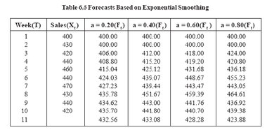
Assume that a firm’s sales over the last 10 weeks are as shown in Table 6.6. By assumption, F2 = Fl = Xl if a = 0.20, then F3 = 0.20(4.30) + 0.80(400) = 406.0 and F4 = 0.20(420) + 0.80(406) = 408.8 The forecasted values for four different values of a are provided in Table 6.6. The table also shows forecasted sales for the next period after the end of the time series data, or week 11. Using a = 0.20, the forecasted sales value for the 11th week is computed to be F11 = 0.20(420) + 0.80(435.7) = 432.56 Table 6.6 suggests why this method is referred to as smoothing technique. Consider the forecasts based on a = 0.20. Note that the smoothed data show much less fluctuation than the original sales data. Note also that as a increases, the fluctuations in the Ft increase, because the forecasts give more weight to the last observed value in the time series.
Choice of a Smoothing Constant
Any value of a could be used as the smoothing constant. One criterion for selecting this value might be the analyst’s intuitive judgment regarding the weight that should be given to more recent data points. But there is also an empirical basis for selecting the value of a. Remember that the coefficients of a regression equation are chosen to minimize the sum of squared deviations between observed and predicted values. This same method can be used to determine the smoothing constant.The term (Xt -Ft)2 is the square of the deviation between the actual time-series data and the forecast for the same period. Thus, by adding these values for eachobservation, the sum of the squared deviations can be computed as observation, deviations can be computed asΣ=−nt 12(X t Ft )One approach to choosing a is to select the value that minimizes this sum. For the data and values of a shown in Table 6.6, these sums are

These results suggest that, of the four values of the smoothing constant, a = 0.60 provides the best forecasts using these data. However, it should be noted that there may be values of a between 0.60 and 0.80 or between 0.40 and 0.60 that yield even better results.
Evaluation of Exponential Smoothing
One advantage of exponential smoothing is that it allows more recent data to begiven greater weight in analyzing time-series data. Another is that, as additional observations become available, it is easy to update the forecasts. There is no needto re-estimate the equations, as would be required with trend projection.The primary disadvantage of exponential smoothing is that it does not provide veryaccurate forecasts if there is a significant trend in the data. If the time trend ispositive, forecasts based on exponential smoothing will be likely to be too low, whilea negative time trend will result in estimates that are too high. Simple exponential smoothing works best when there is no discernable time trend in the data. Thereare, however, more sophisticated forms of exponential smoothing that allow both trends and seasonality to be accounted for in making forecasts.
BAROMETRIC FORECASTING
Barometric forecasting is based on the observed relationships between differenteconomic indicators. It is used to give the decision maker an insight into thedirection of likely future demand changes, although it cannot usually be used to quantify them.Five different types of indicators may be used. Firstly, there are leadingindicators which run in advance of changes in demand for a particular product.An example of these might be an increase in the number of building permits granted which would lead to an increase in demand for building-related productssuch as wood, concrete and so on. Secondly, there are coincident indicatorswhich occur alongside changes in demand. Retail sales would fall into this category,as an increase in sales would generate an increase in demand for themanufacturers of the goods concerned. Thirdly, there are lagging indicatorswhich run behind changes in demand. New industrial investment by firms is often said to fall into this category. In this case it is argued that firms will only invest innew production facilities when demand is already firmly established. Thusincreased investment is a sign, or confirmation, that an initial increase in demand has already taken place. This may well indicate that the economy is improving, forexample, so that further changes in the level of demand can be expected in thenear future.One particular problem with each of these three types of indicator is that singleindicators do not always prove to be accurate in predicting changes in demand. Forthis reason, groups of indicators may be used instead. The fourth and fifth types ofindicator fall into this category. These are composite indices and diffusionindices respectively. Composite indices are made up of weighted averages ofseveral leading indicators which demonstrate an overall trend. Diffusion indices aregroups of leading indicators whose directional shifts are analysed separately. Ifmore than half of the leading indicators included within them are rising, demand is forecast to rise and vice versa. Again, it is important to note that it is the directionof change that is the basis of the prediction, the actual size o of the change cannotbe measured. In addition, the situation is complicated by t the fact that there maybe variations in the length of the lead time between the [various indicators]. This means that the accuracy of predictions may be reduced.
6.7 FORECASTING METHODS: REGRESSION MODELS
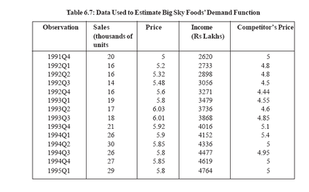
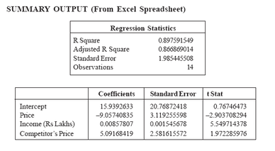
You have seen how regression analysis is used in the estimating process. In thispart you will see several applications of multiple regression analysis to theforecasting process. In this section we shall forecast demand by using data for BigSky Foods (BSF) a company selling groceries.Using the OLS method of estimation available in Excel or any standard statisticalpackage, the demand function we estimated wasQ = 15.939 - 9.057P + .009INC + 5.092PCwhere Q = sales; P = BSF’s price; INC= income; PC = price charged by BSF’smajor competitor. This model can be used to forecast sales, assuming that forecastsof the independent variables are available.
Evaluation of Exponential Smoothing
One advantage of exponential smoothing is that it allows more recent data to begiven greater weight in analyzing time-series data. Another is that, as additional observations become available, it is easy to update the forecasts. There is no needto re-estimate the equations, as would be required with trend projection.The primary disadvantage of exponential smoothing is that it does not provide veryaccurate forecasts if there is a significant trend in the data. If the time trend ispositive, forecasts based on exponential smoothing will be likely to be too low, whilea negative time trend will result in estimates that are too high. Simple exponential smoothing works best when there is no discernable time trend in the data. Thereare, however, more sophisticated forms of exponential smoothing that allow both trends and seasonality to be accounted for in making forecasts.
BAROMETRIC FORECASTING
Barometric forecasting is based on the observed relationships between differenteconomic indicators. It is used to give the decision maker an insight into thedirection of likely future demand changes, although it cannot usually be used to quantify them.Five different types of indicators may be used. Firstly, there are leadingindicators which run in advance of changes in demand for a particular product.An example of these might be an increase in the number of building permits granted which would lead to an increase in demand for building-related productssuch as wood, concrete and so on. Secondly, there are coincident indicatorswhich occur alongside changes in demand. Retail sales would fall into this category,as an increase in sales would generate an increase in demand for themanufacturers of the goods concerned. Thirdly, there are lagging indicatorswhich run behind changes in demand. New industrial investment by firms is often said to fall into this category. In this case it is argued that firms will only invest innew production facilities when demand is already firmly established. Thusincreased investment is a sign, or confirmation, that an initial increase in demand has already taken place. This may well indicate that the economy is improving, forexample, so that further changes in the level of demand can be expected in thenear future.One particular problem with each of these three types of indicator is that singleindicators do not always prove to be accurate in predicting changes in demand. Forthis reason, groups of indicators may be used instead. The fourth and fifth types ofindicator fall into this category. These are composite indices and diffusionindices respectively. Composite indices are made up of weighted averages ofseveral leading indicators which demonstrate an overall trend. Diffusion indices aregroups of leading indicators whose directional shifts are analysed separately. Ifmore than half of the leading indicators included within them are rising, demand is forecast to rise and vice versa. Again, it is important to note that it is the directionof change that is the basis of the prediction, the actual size o of the change cannotbe measured. In addition, the situation is complicated by t the fact that there maybe variations in the length of the lead time between the [various indicators]. This means that the accuracy of predictions may be reduced.
6.7 FORECASTING METHODS: REGRESSION MODELS
You have seen how regression analysis is used in the estimating process. In thispart you will see several applications of multiple regression analysis to theforecasting process. In this section we shall forecast demand by using data for BigSky Foods (BSF) a company selling groceries.Using the OLS method of estimation available in Excel or any standard statisticalpackage, the demand function we estimated wasQ = 15.939 - 9.057P + .009INC + 5.092PCwhere Q = sales; P = BSF’s price; INC= income; PC = price charged by BSF’smajor competitor. This model can be used to forecast sales, assuming that forecastsof the independent variables are available.